Space and Time Complexity Notes
Observing the time complexity of different algorithms


- Space and Time Complexity
- Constant O(1)
- Linear O(n)
- Quadratic O(n^2)
- Logarithmic O(logn)
- Exponential O(2^n)
- Hacks
Space and Time Complexity
Space complexity refers to the amount of memory used by an algorithm to complete its execution, as a function of the size of the input. The space complexity of an algorithm can be affected by various factors such as the size of the input data, the data structures used in the algorithm, the number and size of temporary variables, and the recursion depth. Time complexity refers to the amount of time required by an algorithm to run as the input size grows. It is usually measured in terms of the "Big O" notation, which describes the upper bound of an algorithm's time complexity.
Why do you think a programmer should care about space and time complexity?
-
Space and time complexity are an integral consideration to make about the functionality and running quality of a program. Failing to consider space and time complexity can get in the way of the functionality of the program. Creating bounds for the complexity of a program makes sure that it functions accurately. For example, if time complexity is not considered, then a time-based process that uses the data outputted from a certain long process may fail.
-
There's also a level of convenience for the user to consider. If a program is demanding on a computer and takes a long time to run, people won't want to use it.
Take a look at our lassen volcano example from the data compression tech talk. The first code block is the original image. In the second code block, change the baseWidth to rescale the image.
from IPython.display import Image, display
from pathlib import Path

# prepares a series of images
def image_data(path=Path("images/"), images=None):  # path of static images is defaulted
    for image in images:
        # File to open
        image['filename'] = path / image['file']  # file with path
    return images

def image_display(images):
    for image in images:
        display(Image(filename=image['filename']))

if __name__ == "__main__":
    lassen_volcano = image_data(images=[{'source': "Peter Carolin", 'label': "Lassen Volcano", 'file': "lassen-volcano.jpeg"}])
    image_display(lassen_volcano)

from IPython.display import HTML, display
from pathlib import Path
from PIL import Image as pilImage
from io import BytesIO
import base64

# prepares a series of images
def image_data(path=Path("images/"), images=None):  # path of static images is defaulted
    for image in images:
        # File to open
        image['filename'] = path / image['file']  # file with path
    return images

def scale_image(img):
    baseWidth = 625
    #baseWidth = 1250
    #baseWidth = 2500
    #baseWidth = 5000 # see the effect of doubling or halfing the baseWidth
    #baseWidth = 10000
    #baseWidth = 20000
    #baseWidth = 40000
    scalePercent = (baseWidth/float(img.size[0]))
    scaleHeight = int((float(img.size[1])*float(scalePercent)))
    scale = (baseWidth, scaleHeight)
    return img.resize(scale)

def image_to_base64(img, format):
    with BytesIO() as buffer:
        img.save(buffer, format)
        return base64.b64encode(buffer.getvalue()).decode()

def image_management(image):  # path of static images is defaulted
    # Image open return PIL image object
    img = pilImage.open(image['filename'])

    # Python Image Library operations
    image['format'] = img.format
    image['mode'] = img.mode
    image['size'] = img.size
    # Scale the Image
    img = scale_image(img)
    image['pil'] = img
    image['scaled_size'] = img.size
    # Scaled HTML
    image['html'] = '<img src="data:image/png;base64,%s">' % image_to_base64(image['pil'], image['format'])


if __name__ == "__main__":
    # Use numpy to concatenate two arrays
    images = image_data(images = [{'source': "Peter Carolin", 'label': "Lassen Volcano", 'file': "lassen-volcano.jpeg"}])

    # Display meta data, scaled view, and grey scale for each image
    for image in images:
        image_management(image)
        print("---- meta data -----")
        print(image['label'])
        print(image['source'])
        print(image['format'])
        print(image['mode'])
        print("Original size: ", image['size'])
        print("Scaled size: ", image['scaled_size'])

        print("-- original image --")
        display(HTML(image['html']))

Do you think this is a time complexity or space complexity or both problem?
- I think it's a problem with both. Clearly, since the image wasn't able to display in VSCode and the process ran for around a minute and a half, this is not a well-optimized function for basic laptops.
numbers = list(range(1000))
print(numbers[263])

ncaa_bb_ranks = {1:"Alabama",2:"Houston", 3:"Purdue", 4:"Kansas"}
#look up a value in a dictionary given a key
print(ncaa_bb_ranks[1])
Space
This function takes two integer inputs and returns their sum. The function does not create any additional data structures or variables that are dependent on the input size, so its space complexity is constant, or O(1). Regardless of how large the input integers are, the function will always require the same amount of memory to execute.
def sum(a, b):
  return a + b
Time
An example of a linear time algorithm is traversing a list or an array. When the size of the list or array increases, the time taken to traverse it also increases linearly with the size. Hence, the time complexity of this operation is O(n), where n is the size of the list or array being traversed.
for i in numbers:
    print(i)
Space
This function takes a list of elements arr as input and returns a new list with the elements in reverse order. The function creates a new list reversed_arr of the same size as arr to store the reversed elements. The size of reversed_arr depends on the size of the input arr, so the space complexity of this function is O(n). As the input size increases, the amount of memory required to execute the function also increases linearly.
def reverse_list(arr):
    n = len(arr)
    reversed_arr = [None] * n #create a list of None based on the length or arr
    for i in range(n):
        reversed_arr[n-i-1] = arr[i] #stores the value at the index of arr to the value at the index of reversed_arr starting at the beginning for arr and end for reversed_arr
    return reversed_arr
Time
An example of a quadratic time algorithm is nested loops. When there are two nested loops that both iterate over the same collection, the time taken to complete the algorithm grows quadratically with the size of the collection. Hence, the time complexity of this operation is O(n^2), where n is the size of the collection being iterated over.
for i in numbers:
    for j in numbers:
        print(i,j)
Space
This function takes two matrices matrix1 and matrix2 as input and returns their product as a new matrix. The function creates a new matrix result with dimensions m by n to store the product of the input matrices. The size of result depends on the size of the input matrices, so the space complexity of this function is O(n^2). As the size of the input matrices increases, the amount of memory required to execute the function also increases quadratically.
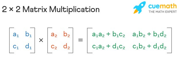
- Main take away is that a new matrix is created.
def multiply_matrices(matrix1, matrix2):
    m = len(matrix1)
    n = len(matrix2[0])
    result = [[0] * n] * m #this creates the new matrix based on the size of matrix 1 and 2
    for i in range(m):
        for j in range(n):
            for k in range(len(matrix2)):
                result[i][j] += matrix1[i][k] * matrix2[k][j]
    return result
Time
An example of a log time algorithm is binary search. Binary search is an algorithm that searches for a specific element in a sorted list by repeatedly dividing the search interval in half. As a result, the time taken to complete the search grows logarithmically with the size of the list. Hence, the time complexity of this operation is O(log n), where n is the size of the list being searched.
def binary_search(arr, low, high, target):
    while low <= high:
        mid = (low + high) // 2 #integer division
        if arr[mid] == target:
            return mid
        elif arr[mid] < target:
            low = mid + 1
        else:
            high = mid - 1

target = 263
result = binary_search(numbers, 0, len(numbers) - 1, target)

print(result)
Space
The same algorithm above has a O(logn) space complexity. The function takes an array arr, its lower and upper bounds low and high, and a target value target. The function searches for target within the bounds of arr by recursively dividing the search space in half until the target is found or the search space is empty. The function does not create any new data structures that depend on the size of arr. Instead, the function uses the call stack to keep track of the recursive calls. Since the maximum depth of the recursive calls is O(logn), where n is the size of arr, the space complexity of this function is O(logn). As the size of arr increases, the amount of memory required to execute the function grows logarithmically.
Time
An example of an O(2^n) algorithm is the recursive implementation of the Fibonacci sequence. The Fibonacci sequence is a series of numbers where each number is the sum of the two preceding ones, starting from 0 and 1. The recursive implementation of the Fibonacci sequence calculates each number by recursively calling itself with the two preceding numbers until it reaches the base case (i.e., the first or second number in the sequence). The algorithm takes O(2^n) time in the worst case because it has to calculate each number in the sequence by making two recursive calls.

def fibonacci(n):
    if n <= 1:
        return n
    else:
        return fibonacci(n-1) + fibonacci(n-2)

#print(fibonacci(5))
#print(fibonacci(10))
#print(fibonacci(20))
print(fibonacci(30))
#print(fibonacci(40))
Space
This function takes a set s as input and generates all possible subsets of s. The function does this by recursively generating the subsets of the set without the first element, and then adding the first element to each of those subsets to generate the subsets that include the first element. The function creates a new list for each recursive call that stores the subsets, and each element in the list is a new list that represents a subset. The number of subsets that can be generated from a set of size n is 2^n, so the space complexity of this function is O(2^n). As the size of the input set increases, the amount of memory required to execute the function grows exponentially.
def generate_subsets(s):
    if not s:
        return [[]]
    subsets = generate_subsets(s[1:])
    return [[s[0]] + subset for subset in subsets] + subsets

print(generate_subsets([1,2,3]))
print(generate_subsets([1,2,3,4,5]))
#print(generate_subsets(numbers))
Using the time library, we are able to see the difference in time it takes to calculate the fibonacci function above.
- Based on what is known about the other time complexities, hypothesize the resulting elapsed time if the function is replaced.
The difference in timing between the functions seems to be based upon the mathematical multipliers associated. For example, in the exponential case below, the time will likely be close to double the previous because the product is continuously multipled by 2 for each n.
For logarithmic, the difference in timing would likely be less extreme as time goes on, since logarithm functions grow longer more than they do greater. It makes sense that quadratic gets greater and greater as n increases, for example.
import time

start_time = time.time()
print(fibonacci(34))
end_time = time.time()

total_time = end_time - start_time
print("Time taken:", total_time, "seconds")

start_time = time.time()
print(fibonacci(35))
end_time = time.time()

total_time = end_time - start_time
print("Time taken:", total_time, "seconds")
Hacks
Below is my work to answer the hacks questions and understand space and time complexity a bit better.
Testing Timing for Remaining Types
Here are some questions and hypotheses I have going in:
- Will the constant's mathematical implications match the difference in processing time?
- Will the exponential processing means be faster than linear at the beginning, but slower when working with larger numbers?
- Is logarithmic most beneficial with larger numbers? Where is the cutoff?
- Where does linear search become slower than binary search?
Using Time Functions
Below are my actual code tests for the duration of each processing algorithm. I decided to use the bodies of code below as samples to test with.
hundnumbers = list(range(100))
tennumbers = list(range(10))
import time

#linear
start_time = time.time()
for num in hundnumbers:
    if num == 90:
        pass
end_time = time.time()

total_time = end_time - start_time
print("Time taken:", total_time, "seconds")

#quadratic
start_time = time.time()
for num in hundnumbers:
    for num2 in hundnumbers:
        if num == 90:
            pass
end_time = time.time()

total_time = end_time - start_time
print("Time taken:", total_time, "seconds")

#logarithmic
start_time = time.time()
binary_search(hundnumbers, 0, 99, 90)
end_time = time.time()

total_time = end_time - start_time
print("Time taken:", total_time, "seconds")

#exponential
start_time = time.time()
fibonacci(90)
end_time = time.time()

total_time = end_time - start_time
print("Time taken:", total_time, "seconds")
import time

#linear
start_time = time.time()
for num in hundnumbers:
    if num == 8:
        pass
end_time = time.time()

total_time = end_time - start_time
print("Time taken:", total_time, "seconds")

#quadratic
start_time = time.time()
for num in hundnumbers:
    for num2 in hundnumbers:
        if num == 8:
            pass
end_time = time.time()

total_time = end_time - start_time
print("Time taken:", total_time, "seconds")

#logarithmic
start_time = time.time()
binary_search(tennumbers, 0, 9, 8)
end_time = time.time()

total_time = end_time - start_time
print("Time taken:", total_time, "seconds")

#exponential
start_time = time.time()
fibonacci(8)
end_time = time.time()

total_time = end_time - start_time
print("Time taken:", total_time, "seconds")
It seems like most of my hypotheses were answered.
- Quadratic processing talkes significantly longer than linear processessing
- Logarithmic is usually faster, but only past around 20 values being tested
- This is an interesting consideration for space complexity
- Exponential is also not that slow until the number gets larger, at which point it gets a lot slower
Hacks Questions
We were asked to answer some questions about time and space complexity. Here are my responses.
- Although we will go more in depth later, time complexity is a key concept that relates to the different sorting algorithms. Do some basic research on the different types of sorting algorithms and their time complexity.
- Why is time and space complexity important when choosing an algorithm?
Time and space complexity are important when choosing an algorithm because they determine how much time and memory an algorithm will require to solve a problem. An algorithm that is efficient in terms of time and space complexity will be faster and require less memory than an algorithm that is not efficient, making it a better choice for solving larger problems or problems that need to be solved quickly.
If the algorithm doesn't work, this is bad from both the perspective of a programmer and of a consumer. A consumer does not want to work with a laggy, slow program that fails to account for large amounts of data and programmers will find it difficult to work around processing algorithms that are very time-consuming.
- Should you always use a constant time algorithm / Should you never use an exponential time algorithm? Explain.
No, you should not always use a constant time algorithm or never use an exponential time algorithm. The choice of algorithm depends on the specific problem being solved and the trade-offs between time and space complexity. In some cases, a constant time algorithm may not be able to solve the problem efficiently, while in other cases, an exponential time algorithm may be the only practical solution. It is important to consider the constraints and requirements of the problem at hand when choosing an algorithm.
- What are some general patterns that you noticed to determine each algorithm's time and space complexity?
Some general patterns to determine time and space complexity are analyzing loops, recursive functions, and nested data structures. For time complexity, counting the number of operations executed by an algorithm related to/caused by the input size is often used to determine time complexity. For space complexity, analyzing the amount of memory required to store data as a function of the input size is often used to determine space complexity.
Time Complexity Analysis Questions
Below are my answers to the linked Time and Space Complexity analysis questions.
Question 1
What is the time and space complexity of the following code?
a = 0
b = 0
for i in range(N):
  a = a + random()

for i in range(M):
  b = b + random()
- O(N * M) time, O(1) space
- O(N + M) time, O(N + M) space
- O(N + M) time, O(1) space
- O(N * M) time, O(N + M) space
My answer: 3 (Correct)
Reasoning: The two for loops are linear O(N) and O(M) respectively, but because they aren't nested, the time complexity isn't described by multiplying N and M. Instead, it would be O(N + M). The variables' sizes are singular and not affected by the size of the input, so the space complexity can be represented as O(1) (linear).
Question 2
What is the time complexity of the following code?
a = 0
for i in range(N):
  for j in reversed(range(i,N)):
    a = a + i + j
- O(N)
- O(N*log(N))
- O(N * Sqrt(N))
- O(N*N)
My answer: 4 (Correct)
Reasoning: These are nested for loops, which were the exact example of quadratic time complexity we learned in class, so I was pretty easily able to identify it as quadratic (O(N*N)).
Question 3
What is the time complexity of the following code?
k = 0
for i in range(n//2, n):
  for j in range(2, n, pow(2,j)):
        k = k + n / 2
- O(n)
- O(nlog(n))
- O(n^2)
- O(n^2(log(n)))
My answer: 2 (Correct)
Reasoning: I really wasn't sure about this one because I found the notation of the range function really confusing. I guess I haven't worked with it enough. I knew the first loop was linear, but the second one seemed like it was doing something like moving up in powers of two, like log with a base of 2. So, the time complexity was O(n * log(2)(n)) or O(nlog(n)).
Question 4
What does it mean when we say that an algorithm X is asymptotically more efficient than Y?
- X will always be a better choice for small inputs
- X will always be a better choice for large inputs
- Y will always be a better choice for small inputs
- X will always be a better choice for all inputs
My answer: 2 (Correct), but we didn't learn what "asymptotically" means
Reasoning: I had to look up "asymptoticallly" to figure it out. Now I know that it means that X is more efficient than Y when a number n is greater than a certain limiting (positive) constant.
Question 5
What is the time complexity of the following code?
a = 0
i = N
while (i > 0):
  a += i
  i //= 2
- O(N)
- O(Sqrt(N))
- O(N / 2)
- O(log N)
My answer: 4 (Correct), but I wasn't confident in it
Reasoning: This was a weird one again because it seemed to resemble the log base 2 example from before, but hasn't been phrased as a while loop yet. Ultimately, I made an educated answer, but not a completely confident one.
Question 6
Which of the following best describes the useful criterion for comparing the efficiency of algorithms?
- Time
- Memory
- Both of the above
- None of the above
My answer: 3 (Correct)
Reasoning: This is just a basic concept that we learned from the lesson.
Question 7
How is time complexity measured?
- By counting the number of algorithms in an algorithm.
- By counting the number of primitive operations performed by the algorithm on a given input size.
- By counting the size of data input to the algorithm.
- None of the above
My answer: 2 (Correct)
Reasoning: This just sounded like a textbook definition, though I didn't know what it meant by "primitive." I knew it wasn't counting the size of the data, and I knew it wasn't as simple as just counting the number of algorithms.
Question 8
What will be the time complexity of the following code?
for i in range(n):
  i=i*k
- O(n)
- O(k)
- O(logk(n))
- O(logn(k))
My answer: 3 (Correct)
Reasoning: Mathematically, it only makes sense to be 3. It couldn't be linear like 1 or 2, since the variable i, which dictates the continued run of the program, is being multiplied by k. In this case, another way to explain the program is that it loops until k has multiplied by itself enough to reach n, which describes how a point would be reached in a logarithmic graph.
Question 9
What will be the time complexity of the following code?
value = 0
for i in range(n):
  for j in range(i):
    value=value+1
- O(n)
- O(n+1)
- O(n(n-1))
- O(n(n+1))
My answer: 4 (Nope)
Correct answer: 3
Reasoning: I had never seen a loop like this before and I wasn't really clear on how I could convert it to Big O notation. Now that I think about it more, range function makes n the ceiling that could never be reached. If n was 2, for example, I would end up being 0 and 1, but never 2. For that reason, O(n * (n - 1)) does make sense.
Question 10
Algorithm A and B have a worst-case running time of O(n) and O(logn), respectively. Therefore, algorithm B always runs faster than algorithm A.
- True
- False
My answer: 2 (Correct)
Reasoning: Part of why I gave this answer is that whenever "always runs faster" is asked in conjunction to a question about time complexity, I will say false. But it's also because, though I'm not familiar with "worst-case running time," I know that linear algorithms (according to my tests) can sometimes be faster with logarithmic ones, especially working with smaller n values.